Pytorch 3 :Model & Training
导言
- 构建复杂模型:学习如何构建更复杂的神经网络模型,如卷积神经网络(CNN)、循环神经网络(RNN)等。
- 损失函数与优化器:理解不同的损失函数(如交叉熵、均方误差)和优化器(如SGD、Adam)。
- 训练与验证:编写训练循环,理解如何监控训练过程,防止过拟合。
神经网络的训练
框架
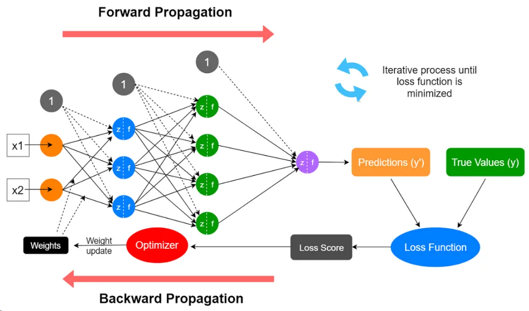
过程大致可以分为以下几步:
- 初始化:对神经网络的权重和偏差进行随机的初始化赋值,将这些初始值作为学习过程的起点;
- 前向传播:输入数据被注入到神经网络中,并通过一系列乘加运算和激活函数,计算每层神经元的激活值,最终产生神经网络的预测输出;
- 损失计算:使用损失函数计算预测输出与实际目标输出之间的差异,量化预测值与真实值的偏差;
- 反向传播:计算损失函数相对于模型参数的梯度,其数值表明损失如何随着这些参数的微小变化而变化;这一步涉及到的数据除了网络中的所有参数外,还需要用到前向传播中计算出来的所有层神经元的激活值;
- 梯度下降:反向传播过程中计算出的梯度表示损失值上升最陡峭的方向,为了最小化损失,网络沿梯度的反方向来更新其参数,更新幅度由学习率控制;
- 迭代:对每一批训练数据(batch)重复步骤2到5多次(epoch),直到神经网络在训练数据上的性能达到令人满意的水平或收敛到一个解决方案。
定义网络
一个简单的前馈神经网络,它接收输入,让输入一个接着一个的通过一些层,最后给出输出。
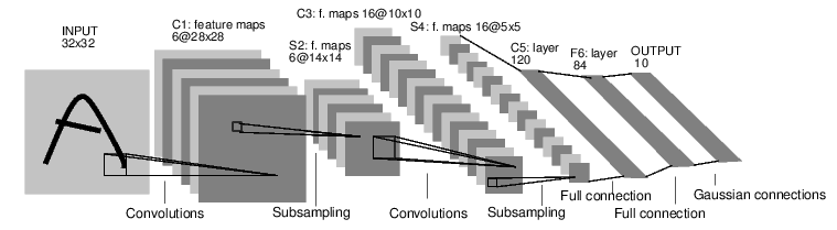 通过 torch.nn 包来构建。一个 nn.Module 包括层和一个方法 forward(input) 它会返回输出(output)。
import torch
import torch.nn as nn
import torch.nn.functional as F


class Net(nn.Module):

    def __init__(self):
        # 习惯上,将包含可训练参数的结构,声明在__init__里
        super(Net, self).__init__()
        # 1 input image channel, 6 output channels, 5x5 square convolution
        # kernel
        self.conv1 = nn.Conv2d(1, 6, 5)
        self.conv2 = nn.Conv2d(6, 16, 5)
        # an affine operation: y = Wx + b
        self.fc1 = nn.Linear(16 * 5 * 5, 120)
        self.fc2 = nn.Linear(120, 84)
        self.fc3 = nn.Linear(84, 10)

    def forward(self, x):
        # Max pooling over a (2, 2) window
        x = F.max_pool2d(F.relu(self.conv1(x)), (2, 2))
        # If the size is a square you can only specify a single number
        x = F.max_pool2d(F.relu(self.conv2(x)), 2)
        x = x.view(-1, self.num_flat_features(x))
        x = F.relu(self.fc1(x))
        x = F.relu(self.fc2(x))
        x = self.fc3(x)
        return x

    def num_flat_features(self, x):
        size = x.size()[1:]  # all dimensions except the batch dimension
        num_features = 1
        for s in size:
            num_features *= s
        return num_features


net = Net()
print(net)
一个模型可训练的参数可以通过调用 net.parameters() 返回:
运行一次网络
梯度累计 和 MicroBatchSize
为了应对batchsize(训练cover的数据量)不够大的问题,将多次迭代的梯度累加后再统一一次反向传播更新。
当你想要的 global batch size 很大,但单卡显存 放不下这么大的 batch 时:
- 把一个大 batch 拆成多个 micro-batch
- 每个 micro-batch 做一次 forward + backward
- 不 step optimizer,只累计梯度
- 累计 N 次后再 optimizer.step()
dataloader = DataLoader(
    dataset,
    batch_size=micro_batch_size,  # 👈 这就是 micro batch
    shuffle=True,
)

optimizer.zero_grad()

for i, batch in enumerate(dataloader): # 不推荐显式chunk,会存储全量激活值,和破坏dataloader的预取和pin_memory逻辑。
    loss = model(batch)
    loss = loss / grad_accum_steps # loss 不要放大了
    loss.backward()

    if (i + 1) % grad_accum_steps == 0:
        torch.nn.utils.clip_grad_norm_(model.parameters(), max_grad_norm = 1.0) # 梯度裁剪,防止爆炸
        optimizer.step()
        optimizer.zero_grad()
Gradient clip norm 超参
梯度还是可能爆, loss / reward 曲线乱跳, 调小来更稳定,但是会学的很慢
学习效率 effective update ≈ min(grad_norm, max_norm) × lr
梯度累计需要适中,让BS/iteration合理
单步BS过大,loss会更稳定,但是泛化性往往会不足。
反向传播计算各个位置梯度
把所有参数梯度缓存器置零,用随机的梯度来反向传播。
一个 optimizer.step() 对应一次 zero_grad()
.backward()是“累加”梯度,不是覆盖梯度。即:param.grad += 当前这次反向得到的梯度- 建议更新完梯度、直接
optimizer.zero_grad()
即使loss是常数,只要loss计算公式能对模型梯度不为0,就能更新权重
- 神经网络只会根据梯度更新。没有梯度,就没有更新。常数 loss 的梯度永远为 0。
梯度取决于“函数形式”是否依赖参数,而不是当前数值是不是常数。
Case
设:
loss 是:
即:
二、求梯度
$$ \nabla_\theta L ===============
\frac{6}{inf_k} \nabla_\theta f(\theta) $$
只要:
梯度就不是 0。
回到danceGRPO,在 θ = θ_old 那个点:ratio = 1 但:
所以模型会开始偏离 1。
损失函数
一个损失函数需要一对输入:模型输出和目标,然后计算一个值来评估输出距离目标有多远。
有一些不同的损失函数在 nn 包中。一个简单的损失函数就是 nn.MSELoss ,这计算了均方误差。
可以调用包,也可以自己设计。
output = net(input)
target = torch.randn(10)  # 随便一个目标
target = target.view(1, -1)  # make it the same shape as output
criterion = nn.MSELoss()

loss = criterion(output, target)
使用loss反向传播更新梯度
查看梯度记录的地方
input -> conv2d -> relu -> maxpool2d -> conv2d -> relu -> maxpool2d
      -> view -> linear -> relu -> linear -> relu -> linear
      -> MSELoss
      -> loss
当我们调用 loss.backward(),整个图都会微分,而且所有的在图中的requires_grad=True 的张量将会让他们的 grad 张量累计梯度。
为了实现反向传播损失,我们所有需要做的事情仅仅是使用 loss.backward()。你需要清空现存的梯度,要不然将会和现存(上一轮)的梯度累计到一起。
查看某处梯度
更新参数(优化器为主)
使用梯度和各种方法优化器更新参数:最简单的更新规则就是随机梯度下降。
我们可以使用 python 来实现这个规则:
尽管如此,如果你是用神经网络,你想使用不同的更新规则,类似于 SGD, Nesterov-SGD, Adam, RMSProp, 等。为了让这可行,我们建立了一个小包:torch.optim 实现了所有的方法。使用它非常的简单。
import torch.optim as optim

# create your optimizer
optimizer = optim.SGD(net.parameters(), lr=0.01)

# in your training loop:
optimizer.zero_grad()   # zero the gradient buffers
output = net(input)
loss = criterion(output, target)
loss.backward()
optimizer.step()    # Does the update
optimizer.zero_grad()
一次到多次训练
一般是按照一次多少batch训练,训练10次等.
或者考虑loss 稳定后结束,一般不使用loss小于某个值(因为不知道loss阈值是多少)
或许可以考虑K折交叉检验法(k-fold cross validation)
for epoch in range(2):  # loop over the dataset multiple times
    running_loss = 0.0
    for i, data in enumerate(trainloader, 0):
        # get the inputs
        inputs, labels = data

        # zero the parameter gradients
        optimizer.zero_grad()

        # forward + backward + optimize
        outputs = net(inputs)
        loss = criterion(outputs, labels)
        loss.backward()
        optimizer.step()

        # print statistics
        running_loss += loss.item()
        if i % 2000 == 1999:    # print every 2000 mini-batches
            print('[%d, %5d] loss: %.3f' %
                  (epoch + 1, i + 1, running_loss / 2000))
            running_loss = 0.0
print('Finished Training')
测试单个任务
分类任务,取最高的
测试总误差
correct = 0
total = 0
with torch.no_grad():
    for data in testloader:
        images, labels = data
        outputs = net(images)
        _, predicted = torch.max(outputs.data, 1)
        total += labels.size(0)
        correct += (predicted == labels).sum().item()

print('Accuracy of the network on the 10000 test images: %d %%' % (
    100 * correct / total))
各种不同的Loss
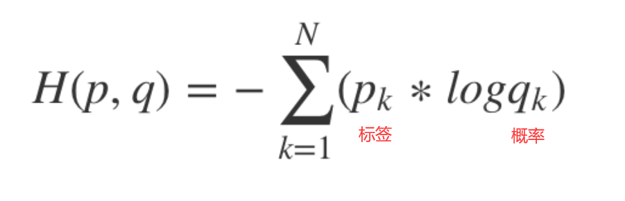
交叉熵和加权交叉熵
多用于多分类任务,预测值是每一类各自的概率。label为特定的类别
 torch.nn.NLLLOSS通常不被独立当作损失函数,而需要和softmax、log等运算组合当作损失函数。
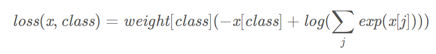
torch.nn.CrossEntropyLoss相当于softmax + log + nllloss。
预测的概率大于1明显不符合预期,可以使用softmax归一,取log后是交叉熵,取负号是为了符合loss越小,预测概率越大。
# 4类权重是 1, 10, 100, 100 一般是与样本占比成反比
criterion = nn.CrossEntropyLoss(weight=torch.from_numpy(np.array([1,10,100,100])).float() ,reduction='sum')
- size_average(该参数不建议使用,后续版本可能被废弃),该参数指定loss是否在一个Batch内平均,即是否除以N。默认为True
- reduce (该参数不建议使用,后续版本可能会废弃),首先说明该参数与size_average冲突,当该参数指定为False时size_average不生效,该参数默认为True。reduce为False时,对batch内的每个样本单独计算loss,loss的返回值Shape为[N],每一个数对应一个样本的loss。reduce为True时,根据size_average决定对N个样本的loss进行求和还是平均,此时返回的loss是一个数。
- reduction 该参数在新版本中是为了取代size_average和reduce参数的。
- 它共有三种选项'mean','sum'和'none'。
- 'mean'为默认情况,表明对N个样本的loss进行求平均之后返回(相当于reduce=True,size_average=True);
- 'sum'指对n个样本的loss求和(相当于reduce=True,size_average=False);
- 'none'表示直接返回n分样本的loss(相当于reduce=False)
Focal Loss
相对于加权交叉熵不仅权重不需要计算,自动通过概率算,而且gamma=2按照平方缩小了,大样本的影响。
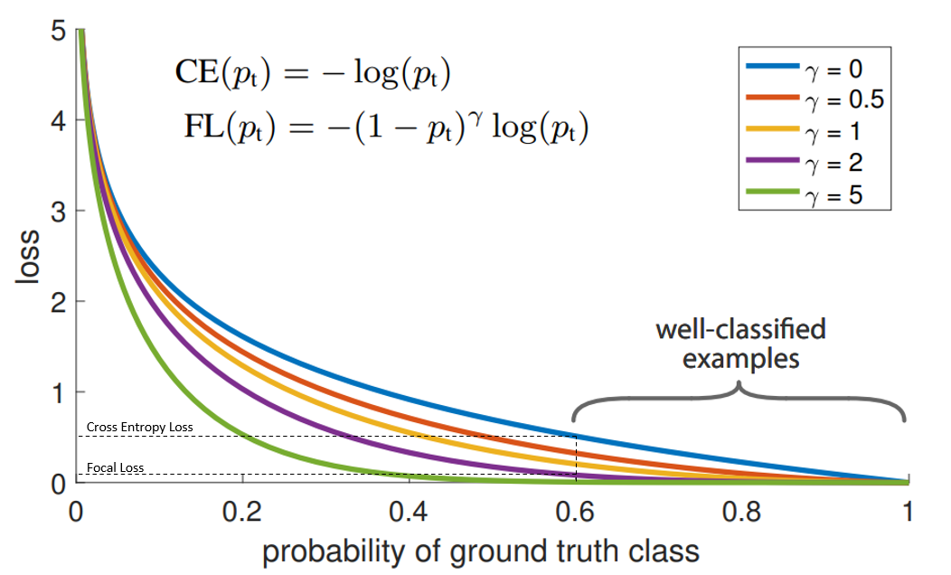
“蓝”线代表交叉熵损失。X轴即“预测为真实标签的概率”(为简单起见,将其称为pt)。举例来说,假设模型预测某物是自行车的概率为0.6,而它确实是自行车, 在这种情况下的pt为0.6。
Y轴是给定pt后Focal loss和CE的loss的值。
从图像中可以看出,当模型预测为真实标签的概率为0.6左右时,交叉熵损失仍在0.5左右。因此,为了在训练过程中减少损失,我们的模型将必须以更高的概率来预测到真实标签。换句话说,交叉熵损失要求模型对自己的预测非常有信心。但这也同样会给模型表现带来负面影响。
深度学习模型会变得过度自信, 因此模型的泛化能力会下降.
当使用γ> 1的Focal Loss可以减少“分类得好的样本”或者说“模型预测正确概率大”的样本的训练损失,而对于“难以分类的示例”,比如预测概率小于0.5的,则不会减小太多损失。因此,在数据类别不平衡的情况下,会让模型的注意力放在稀少的类别上,因为这些类别的样本见过的少,比较难分。
Pytorch.nn常用函数
torch.nn.Linear
设置网络中的全连接层的,需要注意在二维图像处理的任务中,全连接层的输入与输出一般都设置为二维张量,形状通常为[batch_size, size],不同于卷积层要求输入输出是四维张量。
in_features指的是输入的二维张量的大小,即输入的[batch_size, size]中的size。
out_features指的是输出的二维张量的大小,即输出的二维张量的形状为[batch_size,output_size],当然,它也代表了该全连接层的神经元个数。
torch.nn.ReLU()
torch.nn.Sigmoid
- torch.nn.Sigmoid()
- 是一个类。在定义模型的初始化方法中使用,需要在_init__中定义,然后再使用。
- torch.nn.functional.sigmoid():
- 可以直接在forward()里使用。eg.
A=F.sigmoid(x)
torch.cat
cat是concatnate的意思:拼接,联系在一起。
torch.nn.BatchNorm2d
num_features – C from an expected input of size (N, C, H, W)
torch.nn.BatchNorm1d
Input: (N, C) or (N, C, L), where NN is the batch size, C is the number of features or channels, and L is the sequence length
Output: (N, C) or (N, C, L) (same shape as input)
Softmax函数和Sigmoid函数的区别
https://zhuanlan.zhihu.com/p/356976844
钩子函数
EmptyInitOnDevice 类通过重写 torch_function 方法,可以在特定设备上执行某些 PyTorch 操作时修改其行为。具体来说,它可以跳过初始化操作或将新创建的张量放置在指定设备上。torch_function 方法会在每次调用 PyTorch 操作时被触发,从而允许对这些操作进行细粒度的控制。
class EmptyInitOnDevice(torch.overrides.TorchFunctionMode):
    def __init__(self, device=None):
        self.device = device

    def __torch_function__(self, func, types, args=(), kwargs=None):
        kwargs = kwargs or {}
        if getattr(func, '__module__', None) == 'torch.nn.init':
            if 'tensor' in kwargs:
                return kwargs['tensor']
            else:
                return args[0]
        if self.device is not None and func in torch.utils._device._device_constructors() and kwargs.get('device') is None:
            kwargs['device'] = self.device
        return func(*args, **kwargs)
参考文献
https://cloud.tencent.com/developer/article/1669261
https://blog.csdn.net/qq_34914551/article/details/105393989
https://ptorch.com/news/253.html