跳转至

toLearn

3.3 EfficientWorkLearning

科研工作的目标

  1. 从底层的优化做起,自底向上的。对整个AI训练的难点有个全面细致的认知。
  2. 或者从应用的问题出发建模,从上到下有个全面的认知。
  3. 往架构师的方向努力

淡而不厌,简而文,温而理,知远之近,知风之自,知微之显,可与人德矣。

科研学习

狠狠吸收

华为实习部门的都是手握A会的博士大佬。本人望尘莫及,我会狠狠吸收的。

科研的长远与犀利的眼光

  1. 如何识别伪装信息 和被包装的工作
  2. 明确理论目标上限,当前的差距,实现路径

研究理解与实现

  1. 跨领域知识:公众号,订阅
  2. follow前沿论文:follow学者, 公众号,
  3. 实际问题、需求的发现
  4. 技术论证:理论上限,可行方案
  5. 独立任务分割
  6. 高效实现(解决问题)

科研工作的全局观念

  • 自顶向下的设计规划、工作全局观 (从目标、需求、愿景出发。不断细化实现点)
  • 顶:论文全流程思路图(构思与其余工作的对比):当前实现和问题、兼顾创新性的方法 和 设计目标期望效果。
  • 中:代码实现逻辑框架图
  • 底:代码语言具体实现:高内聚低耦合的重要性,解耦,拆分,这样就容易重构了。独立的微服务
  • 自底向上的知识积累 与研究方法提出
  • 底:领域的基础知识
  • 中:领域的主流方法和解决方案
  • 顶:行业痛点和有待补完的领域空白。
  • 当两者相联,目标才能顺利的达成,

高效学习的过程中注意点

  1. 学习的优先级:用20%时间先掌握80%的基础知识或者感兴趣的关键
    1. 难的问题可以讨论合作得出
  2. 提问式主动学习:不是被动学习,尝试通过提问、讨论、教授他人等方式来加深理解和巩固所学内容。
  3. 合作学习: 不仅能头脑风暴idea。对概念的理解,表达能力,心理健康有好处
  4. 交叉与分割学习: 概念文字、视频和案例分析交叉理解。长时间执行单一学习会枯燥,效率降低。切换学习一些新鲜东西:每日关注LLM的有趣实现。
  5. 理论实践交融:实际运行或者编写测试代码运行来深入理解
  6. 持续反馈与评估:每天每周对学习的进度和效果进行分析、来调整学习计划和研究方向。可以遵循STAR 法则。

具体研究点的克服

体系结构量化分析方法,重点就在于量化分析开销,比较然后进行tradeoff。当前前提是你要有基本的相关概念。

具体知识来源的优先级,或者说如何使用搜索引擎:

  1. 明白原理,设计实验,实际机器测量
  2. 认知概念,理解 (图解 >> 列表对比 >> 文字list >> 大段描述)
  3. 阅读相关的论文以及书籍
  4. 国内大佬的博客和大论文
  5. 国外论坛Stack Overflow > 国内知乎 > 博客园 > csdn > 其他
  6. 资料的来源(论文 >> 官方文档 >> 英文博客 >> 高质量中文资料)

在理解概念,量化了具体场景的数值后,就可以开心进行tradeoff了。

  1. 思维导图、摘要,来理清概念 和思路
  2. 结合PPT 数据与图表展示效果

注意项目的可读性和可拓展性一般与性能是不兼容的。这取决于项目的checkpoint/middleValue的保存,在性能优化时往往会消除中间变量。这样会导致代码的可读性和可拓展性下降。

check-point的合理设置

  1. 合理的检查点,既是阶段性的成果,又能在此衍生出无限的可能
  2. 需要能高效的复现与重构

关于如何解决困难

困难的定义可以基于以下几个要素进行评估:

  1. 个人技能能力:困难的程度可以取决于个人所具备的技能和能力水平。对于一个人来说,某项任务可能很容易,而对另一个人来说可能很困难,这取决于他们的专业知识、经验和技能。如果一个人已经具备了必要的知识和技能,那么他们可能更容易应对困难任务。相反,如果缺乏必要的知识和技能,任务就会更具挑战性。
  2. 任务量评估:任务的规模和复杂性也是评估困难程度的重要因素。任务量的多少以及任务本身的复杂性(比如需要解决的问题、涉及的步骤等)会对困难程度产生影响。
  3. 多人合作:效率会由于沟通同步而减半
  4. 量化分析加深理解:对于某些任务,特别是涉及复杂问题解决或决策制定的情况,进行量化分析可以加深对问题本质的理解。这种理解的深度也会对困难程度产生影响,因为解决关键核心会对整个任务的理解的评估进行重大修正。
  5. 对未知领域的任务量评估,会随着了解而变得准确。(这不是产品经理的工作吗?
  6. 时间的紧迫程度:完成任务所要求的时间紧迫程度也是评估困难程度的因素之一。如果任务需要在很短的时间内完成,那么它可能会被认为是更具挑战性和困难的。

参考文献

上面回答部分来自ChatGPT-3.5,没有进行正确性的交叉校验。

3.2 taskPriority

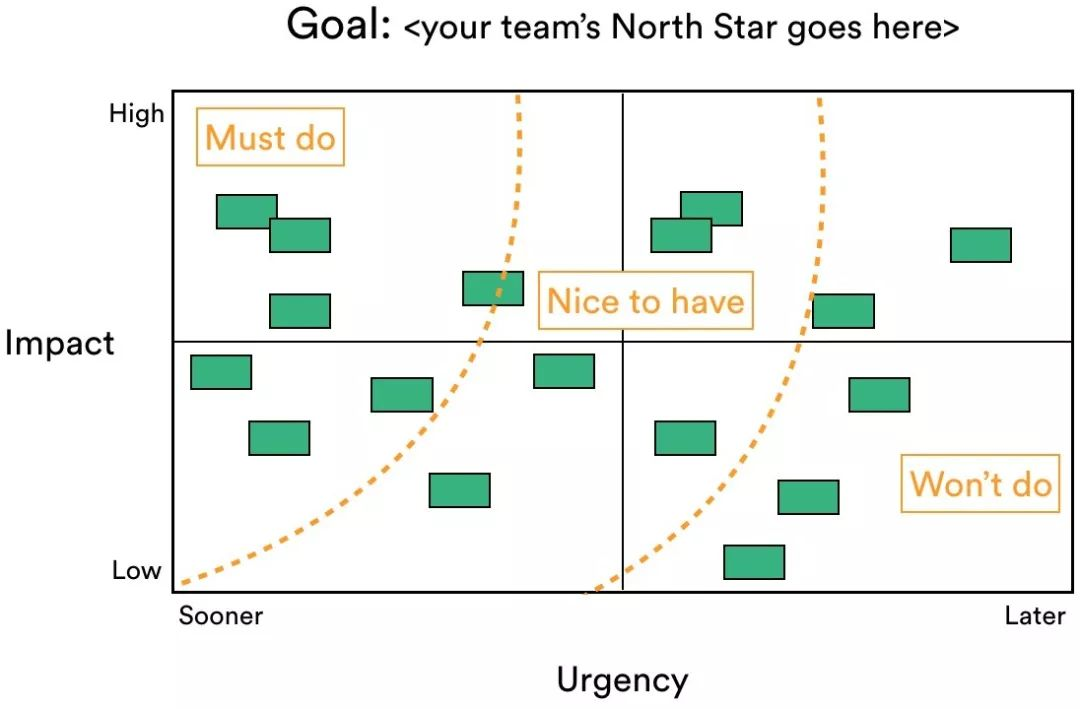
工作优先级四象限(优先级矩阵)

  • 基础版本(艾森豪威尔)
    • 对于紧急又重要的事情马上做。如果这类事情过多,那就想办法规划时间,减少此类事情。
    • 对于重要但不紧急的事情计划做。尽可能地把时间花在重要但不紧急的事情上,这样才能减少产生重要且紧急的工作量。
    • 对于紧急但不重要的事情授权做。处理原则是授权,让别人去做。
    • 最后对于不重要不紧急的事情减少做
  • 额外的维度
    • 依赖关系:工作中显露的潜在工作会打断工作的交付,砍半降低交付效率
      • 尽可能全面

拓展版本

  • 当前工作优先级评估由 四个连续值维度 + 三个逻辑指标 组成
  • 优先级评估的时候不止是自己的视角,还有别人的视角(别人在心里的权重 * 重要性 * 紧迫性)。其中别人在心里的权重,一般来说: 父母、爱人、子女 > 领导 > 我
四个连续值维度
  • 喜好程度
  • 估计工作量(投入收益比)。这一点其实很难量化,自己都没有做怎么知道,只能横向收集友商的数据。
  • 紧急的纬度由DDL时间确定,这点可以和工作量指标互动。
  • 重要性由以下几点确定,都能提高对工作的重要性评价:
    • 增加对工作的喜爱程度的任务: 高效插件与可视化工具的学习使用,
    • 提高工作效率的任务:学习基础知识,
    • 减少长期的工作量:学习、制造和使用轮子;自动化工作。
三个逻辑指标
  • 工作间依赖关系
  • 专注度要求(与疲劳度互补,清醒时才能做思考工作,一天工作后也能进行的简单工程工作)
  • 是否属于未知的领域。(与专注度要求不是正交的关系,是集合的包含关系。需要动脑的事情,肯定是未知的)
经常遇到的实际情况

相同的指标

  1. 紧急程度:不紧急。我一般会比较焦虑,所以工作会较早立项。
  2. 重要程度:我认为重要的才会主动去做,无论是对眼前的毕业考核,还是长远的考虑
  3. 喜好程度:我认为有趣的才会主动去做
  4. 工作间的依赖关系:我会遵守逻辑

不同的指标:

  1. 是否未知:阅读信息的需求
  2. 是否需要专注: 思考需求

两者结合:纯思考 > 阅读加稍微思考 > 初步的阅读收集信息 > 纯机械工作

任务周期内:时间分配和执行顺序

之前的任务优先级评判,都是从完成任务的角度考虑。但是实际情况是每个任务都需要很久(许多任务周期)才能完成。

按照优先级的指标,例如:

紧急性(3) 重要性(3) 喜好(1) 工作量(3) 总分 分配 要求
report 3 0 0 0 3 一天欠 2
thesis 3 3 0 3 9 两天多 3
AI 2 2 1 2 7 两天欠 1
OpenCL 2 1 1 1 5 一天多 1
web 1 0 0 1 2 一天欠 1
Summary 26
  1. 紧急性: 迫在眉睫(几天), 稍等几周,稍等几月,半年一年,可有可无
  2. 重要性: (当下)重大转折,(潜在)深远影响, 一年内小方向,与我无瓜
  3. 喜好:特别喜欢,有点意思,毫无波澜,有点厌恶
  4. 预估工作量(专心情况下):半年以上,一个季度,一个月,一周
  5. 要求(专注度):纯思考 > 阅读加稍微思考 > 初步的阅读收集信息 > 纯机械工作 (3~0)

注意

  • 工作安排 “必须做”占 40%,“愿意做”限制在 30% 左右,剩下30%处理出现的未发现的依赖任务和计划外工作。
  • 涉及到合作的工作:要与对方商量好,自己的选择(为什么把你鸽了,不是)

理想中的二维可视化细节

  • 科研工作与生活各自独立一张图。处理的时间段不同。
  • 横坐标是时间DDL表示紧急程度Urgency,纵坐标是重要性Impact(代表能增强自身和造轮子,还是繁琐小事)
    • 横坐标会随时间自动移动,
    • 标记出四块或者9块颜色
  • 节点可以可视化的部分
    • 颜色深浅表示喜好程度、投入收益比
    • 大小表示工作量绝对值(难易程度)
    • 会根据每日的任务自动调整
    • 甘特图 Gantt:的长条状,中间塞进度条的百分比实现。
    • 和连线表示工作依赖关系
    • 特殊颜色/形状 表示设置里程碑(北极星)任务,完成后自己会收获什么(能力属性标签)
  • 节点额外的属性值(不可视化)
    • 任务的风险
    • 需要的合作者,资源
    • DoD (完成标准,验收标准)
  • 根据公式和数据, 计算工作的优先级并给出推荐。
    • 考虑WIP(Work in Progress)
  • 实现日历功能
  • 为了能激励自身,引入信息增长统计
    • 过去一周/月/季度/年,完成的各类型的Task
    • 引入勤劳值(工作量统计),和收获值(能力增长统计)
    • 能力属性标签, 数值是否随时间衰减

已有的优先级矩阵产品

  • ducalis
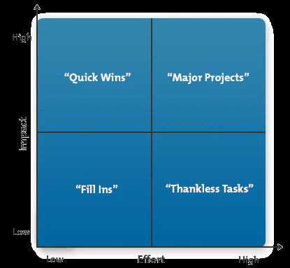
  • 另一种维度,将紧急程度与工作量交换:pic

团队合作的优先级

团队合作中,解决问题的策略与优先级

对象:领导、部门的同事团队( 其余部门的同事团队),个人主体。

思考的基础与前提(多沟通,深分析,找关键):

  1. 找到问题的关键,并提出实用有效的方法
  2. 问题考虑全面,目光长远,设计方法可持续

情形:

  1. 别人遇到问题求助
    1. 授人以鱼不如授人以渔
    2. 如果有其余需求,归纳到最后一点统计决策
  2. 自己遇到问题
    1. 研究瓶颈
      1. 在充分的调研与汇总整理后,向同事或者上级咨询与求助
    2. 两难抉择: 返工的bug修复,新功能,新业务,新研究方向与现有的工作的时间冲突
      1. 工作优先级四象限:根据重要性、紧急程度、喜好程度、工作量(投入收益比)与依赖关系分类
      2. 要与提出需求的对方商量好,解释自己的选择和困难

参考文献

上面回答部分来自ChatGPT-3.5,没有进行正确性的交叉校验。

3 EfficientJumpingRunning

jumping the branch task

五大阻碍工作完成时间的罪魁祸首

  1. 过多的Work in Progress
  2. 太多WIP会导致很多问题:交付延误、品质下降和员工情绪恶化
  3. 利特尔定律 \(\(平均周期时间 =\frac{平均WIP量 }{平均产出量 }\)\)
  4. 未知的依赖工作
  5. 常见依赖关系有3种: > 架构(软件和硬件):一个组件的变更可能破坏另一个组件导致它停止运行 专业知识:从专家那里获得建议或帮助(需要怎样做某事) 活动:直到活动完成才能取得进展
  6. 计划外工作(妨碍你完成某事或导致你无法实现里程碑的干扰事项)
  7. 优先级冲突(相互竞争的项目和任务。当你不确定做什么事情是最重要的时候,就会加剧这种冲突)
  8. 被忽视的工作(技术债)

如何相互影响

  1. 信念/意志确实很重要
  2. 强烈的信念能让你的工作迈出坚实的第一步,而且每一步都走得是否有力
  3. 但是前提是你要十分明确努力的方向,对工作的不自信会减半工作热情。
    1. 工作的优先级冲突,这将导致过多的WIP,从而导致更长的周期时间。
  4. 明确任务的优先级,并分阶段、逐步击破是最好的选择。

需要进一步的研究学习

暂无

遇到的问题

暂无

开题缘由、总结、反思、吐槽~~

参考文献

上面回答部分来自ChatGPT-3.5,没有进行正确性的交叉校验。

DeviceExpansion

拯救者 R7000 2020(1650ti)

内存条

内存为两根8GB DDR4-3200内存组成双通道。 如果要拓展,需要全部升级为 16GB * 2。 拓展视频图文教程

M2固态

可以加装一条2280的固态, 但是无法加机械了。

B450M (主机主板)

内存条

  1. 芯片组最高支持DDR4 2933的内存频率,
  2. 单条内存最大32GB,总容量最大128GB,
  3. 向下可以兼容DDR4 2133、DDR4 2200、DDR4 2400、DDR4 2666。

M2

PCIe 3.0的数据传输速度每通道1GB/s,PCIe 2.0是其一半

B450迫击炮有两个M2插槽,一个是满速pcie3.0×4(4GB/s) 一个是半速的pcie2.0×4(2GB/s)。价格差不多的话还是用M2 nvme协议 的SSD

一点没人提过的,b450m迫击炮装上第二个m2以后,第二个pcie2.0*16的扩展(pcie_4)是没法用的。

需要进一步的研究学习

暂无

遇到的问题

暂无

开题缘由、总结、反思、吐槽~~

参考文献

上面回答部分来自ChatGPT-3.5,没有进行正确性的交叉校验。

Weekly

Content

  1. Background, history
  2. Doing, Situation, Problem, Achievement
  3. Next Plan

year 2023

Weekly 230925-231001

  1. Wednesday 0927
  2. Afternoon: compile and test MultiPIM on icarus0, suffered from python2.7 and lose package dependency. But still encounter pin failed problem

需要进一步的研究学习

暂无

遇到的问题

暂无

开题缘由、总结、反思、吐槽~~

周报是一周的总结和思考,

参考文献

上面回答部分来自ChatGPT-3.5,没有进行正确性的交叉校验。

Wake Up Process

Linux 多进程的竞争休眠机制

基本是基于Linux的时间片轮转机制。A process/thread is woken up by inserting it in the queue of processes/threads to be scheduled.

内核调度算法

CFS(Completely Fair Scheduler)是一种用于 Linux 操作系统的调度算法,它旨在实现对 CPU 时间的公平分配。CFS 是 Linux 内核中默认的调度器,自 Linux 2.6.23 版本以来就成为了标准调度器。

CFS 调度算法的主要目标是确保各个任务在相同的时间片内能够获得公平的CPU时间,不会因为优先级等因素而造成资源争夺不均。以下是 CFS 调度算法的一些关键特点和原则:

  1. 虚拟化时钟: CFS 使用了一种称为虚拟化时钟(virtual runtime)的概念,而不是传统的时间片。每个任务都有一个虚拟运行时间,调度器根据虚拟运行时间来决定哪个任务应该被调度。

  2. 权重: CFS 引入了权重的概念,用于调整不同任务的相对优先级。较高权重的任务会在相同时间间隔内获得更多的虚拟运行时间,从而实现按比例分配CPU资源。

  3. 累积虚拟运行时间: 调度器会根据每个任务的权重和已累积的虚拟运行时间,计算出每个任务的应有的虚拟运行时间片。任务在使用完它的时间片后,会根据虚拟运行时间进行重新排队。

  4. 红黑树结构: CFS 使用红黑树来管理任务队列,这种数据结构使得在插入、删除和搜索任务时的时间复杂度保持在对数级别。

除了 CFS,Linux 内核还有其他调度算法,如:

  • 实时调度器(Real-Time Scheduler): 用于实时任务,提供硬实时和软实时的调度策略,确保实时任务在指定的时间内执行完成。

  • O(1) 调度器(O(1) Scheduler): 是 Linux 2.4 内核中使用的调度器,它的时间复杂度为常数级别。然而,随着多核系统的出现,O(1) 调度器在多核环境下的性能表现受到限制,因此被 CFS 替代。

这些调度算法在不同的场景和需求下,对于多任务操作系统的调度提供了不同的方法和策略。选择适合的调度算法可以根据系统的应用和性能要求来进行。

问题

在高强度竞争之后,有些进程陷入长期sleep,并且在核空闲的时候,也不再重新运行?为什么?

原因可能是程序逻辑阻塞了,或者在等待IO

查看进程Sleep的原因

首先 计算机对一个进程是如何判断sleep的,是某时间内的计算占比低于某个阈值吗?

htop s 可以查看kernel 是不是阻塞, l 可以查看是不是读写同一个文件导致阻塞了。

Sleep的瓶颈在哪里

sleep for what, waiting for what?

实践1 strace

strace -p PID 可以显示一些信息

$ strace -p 4005042
  wait4(-1, # 等待任意子进程结束

# check subprocess
$ pstree -p 4005042
pinbin(4005042)---BC_Compute(4005082)-+-{BC_Compute}(4005187)
                                      |-{BC_Compute}(4005188)
                                      |-{BC_Compute}(4005252)
                                      |-{BC_Compute}(4005296)
                                      |-{BC_Compute}(4005299)
                                      `-{BC_Compute}(4005302)

$ strace -p 4005082
strace: Process 4005082 attached
futex(0x7fffe52de1b8, FUTEX_WAIT, 2, NULL
# futex - fast user-space locking(seems to be used in OpenMP)
# It is typically used as a blocking construct in the context of shared-memory synchronization. 


$ strace -p 4005188
nanosleep({tv_sec=0, tv_nsec=2000000}, 0x7fffe5368bc0) = 0 # repeat
nanosleep({tv_sec=0, tv_nsec=2000000}, 0x7fffe536dbc0) = 0

It seems this is a subprocess repeating sleep leading to all other process to wait in the synchronization.

Use gdb -p PID to attach the process to locate the infinite loop (need Debug Symbols).

futex解释

futex 是 Linux 下的一个系统调用,用于实现用户空间线程间的同步和通信。让我们逐个解释这个系统调用中的每个参数的含义:

  1. 0x7fffe52de1b8: 这是一个指向内存地址的指针(或称为地址),通常是用于表示需要同步的资源或变量的地址。在这里,它表示需要等待的共享资源或变量的地址。
  2. FUTEX_WAIT: 这是一个指定 futex 要执行的操作的标志。FUTEX_WAIT 表示线程正在等待 futex 的值发生变化,即等待条件满足。当某个线程执行 FUTEX_WAIT 操作时,如果 futex 的值与预期不符,则该线程将被置于休眠状态,直到 futex 的值发生变化或超时。
  3. 2: 这是一个表示期望的 futex 值的参数。当调用 FUTEX_WAIT 时,线程将检查 futex 的当前值是否等于此参数指定的值。如果不等于,则线程将休眠等待。
  4. NULL: 这是一个指向 timespec 结构的指针,用于设置超时。这里为 NULL 表示调用没有设置超时,即线程将一直等待,直到 futex 的值发生变化。

总的来说,futex(0x7fffe52de1b8, FUTEX_WAIT, 2, NULL) 表示线程正在等待位于内存地址 0x7fffe52de1b8 的 futex 变量的值等于 2。如果 futex 的值不是 2,则线程将一直等待直到 futex 的值变为 2 或者超时。这样的同步机制在多线程编程中用于等待条件满足后再执行某些操作,从而避免资源竞争和提高程序的并发性能。

nanosleep解释

这是一个系统调用 nanosleep 的输出,通常用于让线程休眠一段时间。让我们逐个解释这个系统调用的含义:

nanosleep({tv_sec=0, tv_nsec=2000000}, 0x7fffe5368bc0) = 0
  1. nanosleep: 这是 Linux 下的一个系统调用,用于使线程休眠一段指定的时间。

  2. {tv_sec=0, tv_nsec=2000000}: 这是传递给 nanosleep 的第一个参数,是一个指向 timespec 结构的指针。timespec 结构用于表示时间间隔,包括秒(tv_sec)和纳秒(tv_nsec)。

在这里,tv_sec=0 表示秒数为 0,tv_nsec=2000000 表示纳秒数为 2000000。因此,这个 nanosleep 调用将会使线程休眠 2 毫秒(1 秒 = 1000000000 纳秒,所以 2000000 纳秒就是 2 毫秒)。

  1. 0x7fffe5368bc0: 这是传递给 nanosleep 的第二个参数,表示一个 timespec 结构的指针。这个参数用于存放未休眠完成的剩余时间,如果 nanosleep 被中断(例如收到信号),它将在这个指针中返回剩余的时间。在这个输出中,剩余时间被存储在内存地址 0x7fffe5368bc0 处。

  2. = 0: 这是 nanosleep 的返回值,表示成功完成。返回值为 0 表示 nanosleep 成功休眠了指定的时间。

综上所述,这个输出表示线程成功休眠了 2 毫秒。

实践2: zsim模拟程序

程序直接执行正常,zsim模拟直接sleep?

$ strace -p 303359
read(10,

$ pstree -p 303359                                                                                 gups_vanilla(303359)-+-gups_vanilla(303449)-+-orted+                                                                    |                      `-{gups+                                                                    |-{gups_vanilla}(303360)                                                                           |-{gups_vanilla}(303361)

$ pstree -p 303449                                                                                 gups_vanilla(303449)-+-orted(303451)-+-{orted}(303452)                                                                  |               |-{orted}(303642)                                                                  |               |-{orted}(303643)                                                                  |               `-{orted}(303644)                                                                  `-{gups_vanilla}(303450)

这是一个 Open MPI(Message Passing Interface)的启动命令,用于启动一个 MPI 程序,并配置一些运行时参数。让我们逐个解释这个命令中的每个选项和参数的含义:

orted --hnp --set-sid --report-uri 11 --singleton-died-pipe 12 -mca state_novm_select 1 -mca ess hnp -mca pmix ^s1,s2,cray,isolated

部分参数含义如下:

  • orted: 这是 Open MPI 的一个工具,用于启动和管理 MPI 进程。
  • -mca state_novm_select 1: 这是一个 MCA(Modular Component Architecture)选项,用于指定某个模块或组件的参数设置。在这里,state_novm_select 设置为 1,可能是指定某个组件或模块在运行时的选项。
  • -mca pmix ^s1,s2,cray,isolated: 这是另一个 MCA 选项,用于配置 PMIx(Process Management Interface for Exascale)的相关设置。^s1,s2,cray,isolated 表示排除 s1、s2、cray 和 isolated 这些模块,可能是禁用某些特定的组件或功能。
pid strace output explanation
303451 restart_syscall(<... resuming interrupted read ...>
303452 futex(0xabba001ec8, FUTEX_WAIT, 2, NULL
303642 epoll_wait(18, ... epoll_wait 系统调用,用于等待文件描述符18上的事件
303643 select(50, [48 49], NULL, NULL, 如下
303644 select(53, [51 52], NULL, NULL,
  • restart_syscall表示系统调用被中断后重新启动的过程。它通常出现在系统调用的执行过程中,当某个信号(例如 SIGSTOP 或 SIGCONT)中断了系统调用的执行,然后系统调用在信号处理完成后被重新启动。
  • select 是一个用于在多个文件描述符上进行 I/O 多路复用(I/O multiplexing)的系统调用,它可以监视多个文件描述符,并在其中任何一个文件描述符准备好进行 I/O 操作时返回。
  • select 调用的输出,它将监视文件描述符 48 和 49,并在其中任何一个文件描述符准备好读取数据或超时(2 秒后)时返回。
  • 完全无法理解呢! 可能需要深入了解MPI的实现栈细节才能明白。

命令行唤醒Sleep进程

The only way to “wake it up” is to arrange for the condition to be met. 用户是无法更改的状态的。

传统kill进程

# find pid , state S+ meaning sleep
ps aux | grep name
# gracefully kill process
kill -15 pid

需要进一步的研究学习

暂无

遇到的问题

暂无

开题缘由、总结、反思、吐槽~~

参考文献

上面回答部分来自ChatGPT-3.5,没有进行正确性的交叉校验。

Benchmark

Differentiated-Bounded Applications

According to the DAMOV, data movement have six different types.

Although the authors only use temporal Locality to classify the apps, the Figure 3: Locality-based clustering of 44 representative functions shows some cases deserved to test.

In the context of data movement, the DAMOV framework identifies six distinct types. While the authors primarily utilize temporal locality for app classification, Figure 3 offers a comprehensive view of the locality-based clustering of 44 representative functions, highlighting specific cases that warrant further examination.

Take, for instance, the four cases situated in the lower right corner:

function short name benchmark class
CHAHsti Chai-Hito 1b: DRAM Latency
CHAOpad Chai-Padding 1c: L1/L2 Cache Capacity
PHELinReg Phoenix-Linear Regression 1b
PHEStrMat Phoenix-String Matching 1b

TLB percentage high -> tlb miss rate high -> memory access address in large span -> spacial locality is low.

benchmark

Chai Benchmark

The Chai benchmark code can be sourced either from DAMOV or directly from its GitHub repository. Chai stands for "Collaborative Heterogeneous Applications for Integrated Architectures."

Installing Chai is a straightforward process. You can achieve it by executing the command python3 compile.py.

One notable feature of the Chai benchmark is its adaptability in terms of input size. Modifying the input size of the following applications is a simple and flexible task:

# cd application directory
./bfs_00 -t 4 -f input/xxx.input
./hsti -n 1024000             # Image Histogram - Input Partitioning (HSTI)
./hsto -n 1024000             # Image Histogram - Output Partitioning (HSTO)
./ooppad -m 1000 -n 1000   # Padding (PAD)
./ooptrns -m 100 -n 10000  # Transpose / In-place Transposition (TRNS)
./sc -n 1024000            # Stream Compaction (SC)
./sri -n 1024000           # select application

# vector pack , 2048 = 1024 * 2, 1024 = 2^n
./vpack -m 2048 -n 1024 -i 2 
# vector unpack , 2048 = 1024 * 2, 1024 = 2^n
./vupack -m 2048 -n 1024 -i 2 

Parboil (how to run)

The Parboil suite was developed from a collection of benchmarks used at the University of Illinois to measure and compare the performance of computation-intensive algorithms executing on either a CPU or a GPU. Each implementation of a GPU algorithm is either in CUDA or OpenCL, and requires a system capable of executing applications using those APIs.

# compile , vim compile.py 
# python2.7 ./parboil compile bfs omp_base 
python3 compile.py

# no idea how to run, failed command: (skip)
python2.7 ./parboil run bfs cuda default 
# exe in benchmarks/*, but need some nowhere input.

Phoenix

Phoenix is a shared-memory implementation of Google's MapReduce model for data-intensive processing tasks.

# with code from DAMOV
import os
import sys

os.chdir("phoenix-2.0/tests") # app is changed from sample_apps/*
os.system("make")
os.chdir("../../")

# generate excution in phoenix-2.0/tests/{app}/{app}

# running for example
./phoenix-2.0/tests/linear_regression/linear_regression ./phoenix-2.0/datasets/linear_regression_datafiles/key_file_500MB.txt 

PolyBench

PolyBench is a benchmark suite of 30 numerical computations with static control flow, extracted from operations in various application domains (linear algebra computations, image processing, physics simulation, dynamic programming, statistics, etc.).

PolyBench features include:

  • A single file, tunable at compile-time, used for the kernel instrumentation. It performs extra operations such as cache flushing before the kernel execution, and can set real-time scheduling to prevent OS interference.
# compile using DAMOV code
python compile.py
# exe in OpenMP/compiled, and all running in no parameter

PriM

real apps for the first real PIM platform

Rodinia (developed)

Rodinia, a benchmark suite for heterogeneous parallel computing which target multi-core CPU and GPU platforms, which first introduced in 2009 IISWC.

zsim hooked code from github

  1. Install the CUDA/OCL drivers, SDK and toolkit on your machine.
  2. Modify the common/make.config file to change the settings of
  3. rodinia home directory and CUDA/OCL library paths.
  4. It seems need intel opencl, but intel do everything to oneapi
  5. To compile all the programs of the Rodinia benchmark suite, simply use the universal makefile to compile all the programs, or go to each benchmark directory and make individual programs.
  6. full code with related data can be downloaded from website
mkdir -p ./bin/linux/omp
make OMP

Running the zsim hooked apps

cd bin/linux/omp
./pathfinder 100000 100 7
./myocyte.out 100 1 0 4
./lavaMD -cores 4 -boxes1d 10 # -boxes1d  (number of boxes in one dimension, the total number of boxes will be that^3)
./omp/lud_omp -s 8000
./srad 2048 2048 0 127 0 127 2 0.5 2
./backprop 4 65536 # OMP_NUM_THREADS=4


# need to download data or file
./hotspot 1024 1024 2 4 ../../data/hotspot/temp_1024 ../../data/hotspot/power_1024 output.out
./OpenMP/leukocyte 5 4 ../../data/leukocyte/testfile.avi
# streamcluster
./sc_omp k1 k2 d n chunksize clustersize infile outfile nproc
./sc_omp 10 20 256 65536 65536 1000 none output.txt 4
./bfs 4 ../../data/bfs/graph1MW_6.txt 
./kmeans_serial/kmeans -i ../../data/kmeans/kdd_cup
./kmeans_openmp/kmeans -n 4 -i ../../data/kmeans/kdd_cup

dynamic data structures

We choose this specific suite because dynamic data structures are the core of many server workloads (e.g., Memcached’s hash table, RocksDB’s skip list), and are a great match for nearmemory processing

ASCYLIB + OPTIK1

Graph Apps

Graph500 Benchmark Exploration

Official Version

The official version of the Graph500 benchmark can be downloaded from its GitHub repository. Notable features of this version include:

  • Primarily MPI Implementation: The benchmark is built as an MPI (Message Passing Interface) version, without an accompanying OpenMP version. This can be disappointing for those utilizing tools like zsim.
  • Flexible n Value: By default, the value n is set to powers of 2, but it's possible to change this behavior through configuration adjustments.
  • Customization Options: Environment variables can be altered to modify the execution process. For instance, the BFS (Breadth-First Search) portion can be skipped or the destination path for saved results can be changed.
Unofficial Repository

An alternative unofficial repository also exists. However, it requires OpenCL for compilation. The process can be broken down as follows:

  • OpenCL Dependency: The unofficial repository mandates the presence of OpenCL. To set up OpenCL, you can refer to this tutorial.
sudo apt-get install clinfo
sudo apt-get install opencl-headers
sudo apt install opencl-dev

After completing the OpenCL setup and the compilation process using cmake & make, we obtain the executable file named benchmark. By default, running this executable without any arguments appears to utilize only a single core, despite attempts to set the environment variable with export OMP_NUM_THREADS=32. This default behavior led to a runtime of approximately 5 minutes to generate a report related to edges-node-verify status (or similar). However, for someone without an in-depth technical background, this report can be confusing, especially when trying to locate the BFS (Breadth-First Search) and SSSP (Single-Source Shortest Path) components.

What is even more disheartening is that the TLB (Translation Lookaside Buffer) result is disappointingly low, similar to the performance of the GUPS (Giga Updates Per Second) OpenMP version.

In order to gain a clearer understanding and potentially address these issues, further investigation and potentially adjustments to the program configuration may be necessary.

$ ./tlbstat -c '/staff/shaojiemike/github/graph500_openmp/build/benchmark' 
command is /staff/shaojiemike/github/graph500_openmp/build/benchmark                       
K_CYCLES   K_INSTR      IPC DTLB_WALKS ITLB_WALKS K_DTLBCYC  K_ITLBCYC  DTLB% ITLB%         
20819312   10801013    0.52 7736938    1552557    369122     51902       1.77  0.25
20336549   10689727    0.53 7916323    1544469    354426     48123       1.74  0.24

GAP

Zsim?/LLVM Pass Instrumentation Code from PIMProf paper github

But the graph dataset should be generated by yourself following the github:

# 2^17 nodes 
./converter -g17 -k16 -b kron-17.sg
./converter -g17 -k16 -wb kron-17.wsg

Kernels Included

  • Breadth-First Search (BFS) - direction optimizing
  • Single-Source Shortest Paths (SSSP) - delta stepping
  • PageRank (PR) - iterative method in pull direction
  • Connected Components (CC) - Afforest & Shiloach-Vishkin
  • Betweenness Centrality (BC) - Brandes
  • Triangle Counting (TC) - Order invariant with possible relabelling

ligra

Code also from DAMOV

# compile
python3 compile.py

# 3 kind exe of each app, relative code can be found in /ligra directory
# emd: edgeMapDense() maybe processing related dense-data 
# ems: edgeMapSparse() analyse edge-data
# compute: of course, the core compute part

the source code is difficult to read, skip

the graph format : It seems lines_num = offsets + edges + 3

AdjacencyGraph
16777216 # offsets, and vertex from []
100000000 #   uintE* edges = newA(uintE,m);
0
470
794 # must monotonic increasing, and range [0,edges), represent the folloing edges are belong to corresponding vector
……
14680024 # random but range [0,vector-1], represent each node's conjoint others nodes(so there are pairs).
16644052
16284631
15850460

$ wc -l  /staff/qcjiang/codes/DAMOV/workloads/ligra/inputs/rMat_10M
116777219 /staff/qcjiang/codes/DAMOV/workloads/ligra/inputs/rMat_10M

Pagerank Algorithm should be referened from my another post.

HPC

maybe more computation-intensive than graph applications

parsec

From DAMOV

The Princeton Application Repository for Shared-Memory Computers (PARSEC) is a collection of parallel programs which can be used for performance studies of multiprocessor machines.

# compile
python3 compile_parsec.py

# exe in pkgs/binaries
./pkgs/binaries/blackscholes 4 ./pkgs/inputs/blackscholes/in_64K.txt black.out
./pkgs/binaries/fluidanimate 4 10 ./pkgs/inputs/fluidanimate/in_300K.fluid

STREAM apps

DAMOV code for memory bandwidth testing which reference J. D. McCalpin et al., “Memory Bandwidth and Machine Balance in Current High Performance Computers,” IEEE TCCA Newsletter, 1995

# compile
python3 compile.py

# default run with Failed Validation error(whatever)
-------------------------------------------------------------
Function    Best Rate MB/s  Avg time     Min time     Max time
Copy:            5072.0     0.205180     0.157728     0.472323
Add:             6946.6     0.276261     0.172746     0.490767

Hardware Effects

Two very Interesting repositys of cpu and gpu hardware effects that can degrade application performance in surprising ways and that may be very hard to explain without knowledge of the low-level CPU/GPU and OS architecture.

Test also using DAMOV code

# compile
python3 compile.py

# Every example directory has a README that explains the individual effects.
./build/bandwidth-saturation/bandwidth-saturation 0 1
./build/false-sharing/false-sharing 3 8

Most cases using the help of perf to know more about your system ability.

HPCC

From DAMOV and The HPC Challenge (HPCC) Benchmark Suite,” in SC, 2006

  • RandomAccess OpenMP version (it is also the GUPS)
# install
python compile.py

# must export
export OMP_NUM_THREADS=32
./OPENMP/ra_omp 26 # 26 need almost 20GB mem, 27 need 30GB mem, and so on.

but the openmp version shows no big pgw overhead

GUPS

描述系统的随机访问能力

From github or hpcc official-web and RandomAccess MPI version

# download using github
make -f Makefile.linux gups_vanilla
# running
gups_vanilla N M chunk
  • N = length of global table is 2^N
  • Thus N = 30 would run with a billion-element table.
  • M = # of update sets per proc 越大代表算得越久(随机访问越久),
  • chunk = # of updates in one set on each proc
  • In the official HPCC benchmark this is specified to be no larger than 1024, but you can run the code with any value you like. Your GUPS performance will typically decrease for smaller chunk size.

测试之后,最佳搭配如下 mpirun -n 32 ./gups_vanilla 32 100000 2048 其中n最多32,不然会爆内存。

n 32 31 30 29
DTLB% 66.81 45.22 19.50 13.20
ITLB% 0.06 0.07 0.06 0.09

或者单独运行./gups_vanilla 30 100000 k (n最多30), ./tlbstat -c '/usr/bin/mpirun -np 1 /staff/shaojiemike/github/gups/gups_vanilla 30 100000 8192

n\k 1024 2048 4096 8192
30 44% 90% 80%
27 88%
24 83% 83%
20 58% 62%
15 0.27% 0.3%
手动构造 bigJump
#include <bits/stdc++.h>
#include "../zsim_hooks.h"
using namespace std;

#define MOD int(1e9)

// 2000 tlb entries is the normal cpu config, 
// for 4KB page, each data access trigers tlb miss, jump over 1000 int, 
// and after 2000 entries to repeat, so at least 2000 * 4KB = 8MB space

// #define BASIC_8MB 2000000 * 2
#define BASIC_8MB (1 << 22)

// 1 second program. stream add 6GB/s, int is 4B, repeated 10^9
// #define all_loops 1000000
#define all_loops (1 << 20)

int main(int argc, char* argv[]) {
   if (argc != 4) {
      std::cerr << "Usage: " << argv[0] << " <space scale> <jump distance scale> <loop times>" << std::endl;
      return 1;
   }

   // Convert the second command-line argument (argv[1]) to an integer
   int N = std::atoi(argv[1]);
   int J = std::atoi(argv[2]);
   int M = std::atoi(argv[3]);

   std::cout << "Number read from command line: " << N << " " << J << " (N,J should not big, [0,5] is best.)" <<std::endl;

   const int size = BASIC_8MB << N;
   const int size_mask = size - 1;
   int * jump_space = (int *)malloc(size * sizeof(int));

   zsim_begin();
   int result = 0;
   int mem_access_count = 0;
   int mem_access_index = 0;
   // int mask = (1<<10<<J)-1;
   // int ran = 0x12345678;
   int mask = (1<<J)-1;
   int ran = (1<<30)-1;
   // without random address, tlb occupancy is alse high
   // ran = (ran << 1) ^ ((int) ran < 0 ? 0x87654321 : 0);
   while(mem_access_count++ < all_loops*M){
      // read & write 
      jump_space[mem_access_index] = ran;
      mem_access_index = (mem_access_index + (1024 + ran & mask) ) & (size_mask);
      // cout << "mem_access_index = " << mem_access_index << endl;
   }
   zsim_end();

   //print first 5 elements
   printf("result %d",result);
}

HPCG

From DAMOV and High Performance Conjugate Gradient Benchmark (HPCG)

HPCG is a software package that performs a fixed number of multigrid preconditioned (using a symmetric Gauss-Seidel smoother) conjugate gradient (PCG) iterations using double precision (64 bit) floating point values. 浮点数的共轭梯度求解

follow the instructions in INSTALL and analyze the compile.py

  1. choose makefile like setup/Make.GCC_OMP
  2. config values like MPdir, but we can leave them beacuse we use GCC_OMP which set -DHPCG_NO_MPI in it
  3. add -DHPGSym to CXXFLAGS or HPCG_OPTS
  4. cd build and ../configure GCC_OMP
  5. run compile.py to compile the executable files
  6. get 4 ComputePrologation in build/bin
  7. test the exe using xhpcg 32 24 16 for three dimension
  8. or xhpcg --nx=16 --rt=120 for NX=NY=NZ=16 and time is 120 seconds
  9. change int refMaxIters = 50; to int refMaxIters = 1; to limit CG iteration number
  10. to be attention: --nx=16 must be a multiple of 8
  11. if there is no geometry arguments on the command line, hpcg will ReadHpcgDat and get the default --nx=104 --rt=60
value\nx 96 240 360 480
mem 17GB 40GB 72.8GB
time(icarus0) 8s 84S 4min40s core dumped(7mins)

core dumped for xhpcg_HPGPro: ../src/GenerateProblem_ref.cpp:204: void GenerateProblem_ref(SparseMatrix&, Vector*, Vector*, Vector*): Assertion 'totalNumberOfNonzeros>0' failed.

MPdir        = 
MPinc        = 
MPlib        = 

HPCG_OPTS     = -DHPCG_NO_MPI -DHPGSym
compile error
../src/ComputeResidual.cpp:59:13: error: 'n' not specified in enclosing 'parallel'

just add n to shared values

Database

Hash Joins

This package provides implementations of the main-memory hash join algorithms described and studied in C. Balkesen, J. Teubner, G. Alonso, and M. T. Ozsu, “Main-Memory Hash Joins on Modern Processor Architectures,” TKDE, 2015.

Test also in DAMOV

# install
python compile.py

# runing
./src/mchashjoins_* -r 12800000 -s 12000000 -x 12345 -y 54321

these case shows tlb resource strains

AI

Darknet for CV using multi-cores

From DAMOV and official documentation is detailed

shaojiemike @ snode6 in ~/github/DAMOV/workloads/Darknet on git:main x [14:13:02]                   │drwxr-xr-x  3 shaojiemike staff   21 Mar 14  2022 .
$ ./darknet detect cfg/yolo.cfg ./weights/yolo.weights data/dog.jpg
  • model in weight files, different size model (28MB -528MB)can be downloaded from website
  • picture data in data files. (70KB - 100MB)
  • must run the exe in the file directory. SHIT.

genomics / DNA

BWA

From DAMOV and for mapping DNA sequences against a large reference genome, such as the human genome

  • Download DNA data like ref.fa following Data download steps
  • stucked when running sratoolkit.3.0.6-ubuntu64/bin/fastq-dump --split-files SRR7733443 due to generate several 96GB SRR7733443_X.fastq files which X from 1 to n.
  • sratool can not limit the file size, but we can use head -c 100MB SRR7733443_1.fastq > ref_100MB.fastq to get wanted file size.
  • Further running commands you can read the github
  • ./bwa index -p abc ref_100MB.fastq will generate sevaral abc.suffix files using 50 seconds.
  • and now you can run ./bwa mem -t 4 abc ref_100MB.fastq or ./bwa aln -t 4 abc ref_100MB.fastq

GASE

GASE - Generic Aligner for *Seed-and-Extend


GASE is a DNA read aligner, developed for measuring the mapping accuracy and execution time of different combinations of seeding and extension techniques. GASE is implemented by extending BWA (version 0.7.13) developed by Heng Li.

Code also from DAMOV. But seems there are some program syntax errors, skip this app.

需要进一步的研究学习

暂无

遇到的问题

暂无

开题缘由、总结、反思、吐槽~~

参考文献

DAMOV: A New Methodology and Benchmark Suite for Evaluating Data Movement Bottlenecks

Jupyter AI

Jupyter 简介

Jupyter是一个开源的、交互式的计算环境,可以让用户创建和共享包含实时代码、可视化和文本的文档。

  • 它的名字来源于三个主要的编程语言:Julia、Python和R,这三种语言的开头字母构成了“Jupyter”。
  • Jupyter最初是IPython项目的一部分,旨在提供Python的交互式计算环境。随着时间的推移,它不仅支持Python,还扩展到其他编程语言,包括R、Julia、Scala等。Jupyter的灵感来自于IPython的交互式shell,但在其基础上增加了更多功能和可扩展性。

Jupyter最显著的特点:用户可以通过Web浏览器打开Jupyter笔记本,然后在其中编写代码、运行代码并直接查看代码的输出结果。笔记本中的代码和文本可以交叉编排,使得写作、数据分析和可视化变得非常直观和便捷。

主要的Jupyter组件包括:

  1. Jupyter Notebook:这是最常见的Jupyter界面,以.ipynb后缀的文件保存。它支持多种编程语言的代码运行,交互式地执行和编辑代码块,并支持在代码块中插入Markdown格式的文本以及图像、链接等内容。
  2. Jupyter Lab:这是Jupyter Notebook的下一代界面,提供了更加现代化和灵活的界面。Jupyter Lab将各种组件整合到一个集成的界面中,使得多个笔记本、终端和文件浏览器可以在一个窗口中同时运行。
  3. Jupyter Kernel:Jupyter支持多种编程语言的内核,通过内核,Jupyter可以与特定编程语言进行交互。例如,使用Python内核可以在笔记本中运行和编写Python代码,同样,使用R内核可以运行和编写R代码。

Jupyter在教育、数据科学、机器学习、数据分析等领域得到广泛应用。它提供了一个方便、实用的平台,帮助用户探索数据、实验算法、展示结果,并通过共享笔记本方便地与其他人交流和合作。

Jupyter vs python

Jupyter 的核心在于 数据分析的 计算-分析-可视化 的快速迭代。

如果不是数据科学,就不太需要Jupyter

Installation in Linux

安装Jupyter Lab

web-forward to local machine

远程访问服务器

Jupyter-AI

  1. Installation
  2. test

需要进一步的研究学习

暂无

遇到的问题

暂无

开题缘由、总结、反思、吐槽~~

  1. python 一大特点就是容易可视化,既然这样,我为什么不用jupyter呢?
  2. chatgpt 类的工具都是基于付费API,有两大问题
  3. 国内难以付费
  4. 国内ip一旦访问是很容易封号的。
  5. 一种解决办法是使用有免费API的工具,并且在全流量走cloudflare的wg的服务器上配置服务。

参考文献

上面回答部分来自ChatGPT-3.5,没有进行正确性的交叉校验。

https://jupyter-ai.readthedocs.io/en/latest/users/index.html#installation

Parallel_sort

并行排序算法

to learn

PSRS算法

并行正则采样排序算法

PSRS

复杂度分析

简单地讨论一下 PSRS 算法的复杂度。

  • 在第一部分的快速排序中,时间复杂度为O(klogk),k=n/p
  • 然后,各处理器选择 p-1 个代表元素,代价为O(p)
  • 再由 Proc#0 对所有送来的代表元素进行排序,然后选出主元,这里若使用快速排序,代价为O(p^2 logp^2)
  • 而若使用归并排序,则所需代价为O(p^2)
  • 每个处理器接收到主元后,再对有序数组进行划分,代价为O(k+p)
  • 最后,各个处理器全局交换,并行归并排序,
  • 每个处理器是串行的多路归并问题,时间复杂度为O(k*logp)

考虑到实际应用中,需要排序的数据长度 n 一定远远多于现有的处理器 p,此时可以视 p 为一个小常数,那么 PSRS 排序算法的时间复杂度,就可以简化为 O(klogk+k*logp)~O(klogk)

从消息复杂度的角度看,

  • 播送主元的复杂度为 O(p^2+p)
  • 分区合并(全局交换)部分的消息复杂度与具体算法实现相关,但其最大值不会超过 O(n)

需要进一步的研究学习

暂无

遇到的问题

暂无

开题缘由、总结、反思、吐槽~~

参考文献

上面回答部分来自ChatGPT-3.5,没有进行正确性的交叉校验。

https://dingfen.github.io/mpi&openmp/2021/01/23/psrs_sort.html